Machine Description case
In this example we will combine multiple IMAS-ParaView non-GGD plugins to read ITER machine description data. We will create an animation where we orbit the camera around the machine description data, so we can see the different structures clearly from every angle.
You can download the ParaView state file for this example here. However, we recommend that you manually follow the steps outlined below.
Loading the Wall data
In this subsection, we will visualize the divertor and first wall structures, and create a rotational extrusion to rotate them around the central axis.
Navigate to Sources > IMAS Tools and select the Wall Limiter Reader.
Enter the following URI in the
Enter URIfield of the Wall Limiter reader plugin:imas:hdf5?path=/work/imas/shared/imasdb/ITER_MACHINE_DESCRIPTION/3/116000/5Since this URI only contains a single supported IDS for this reader, the wall IDS, it is automatically selected for you. You should see the Divertor and First Wall attributes appear in the attribute array selection, select them both.
Select
Applyto load the Divertor and First Wall structures.After the structures are loaded, bring them into view by aligning the viewpoint in the positive Y direction using the following button:
 .
.We will now rotate the divertor and first wall around the central axis. For this, we will use the Rotational Extrusion filter. Select the Filters > Search... menu, type
Rotational Extrusionand select the filter.Set the resolution to 50, and the angle to 360. Press
Applyto apply the rotational extrusion filter.We will now fix the legend labels for the blocks, select
Editunder the coloring section and remove all the categories for numbers higher than 1, and select the minus icon.Now rename the annotations for the 0 and 1 blocks to
DivertorandFirst Wall, respectively.Lastly, set the opacity to 0.5, so we can view the inside of the wall.
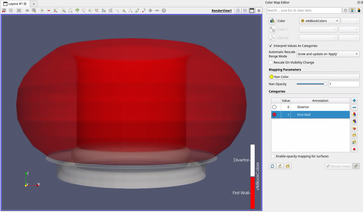
The first wall and divertor structures extruded around the center axis. Data provided by X. Bonnin.
Loading the EC launcher beams
Navigate to Sources > IMAS Tools and select the Beam Reader.
Enter the following URI in the
Enter URIfield of the Beam reader plugin:imas:hdf5?path=/work/imas/shared/imasdb/ITER_MACHINE_DESCRIPTION/3/120000/1304Since this URI only contains a single supported IDS for this reader, the ec_launchers IDS, it is automatically selected for you. You should see the EC launcher beam names appear in the attribute array selection, select them all, and press
Apply.Change the color of the beams to a color of choosing, by pressing
Editunder the coloring options. Here we use cyan.
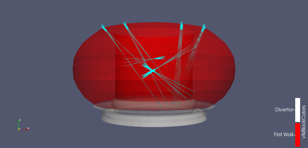
The EC launcher beams are added in cyan. Data provided by M. Schneider.
Loading the Interferometer lines of sight
Navigate to Sources > IMAS Tools and select the Line of Sight Reader.
Enter the following URI in the
Enter URIfield of the Line of Sight reader plugin:imas:hdf5?path=/work/imas/shared/imasdb/ITER_MACHINE_DESCRIPTION/3/150610/2Since this URI only contains a single supported IDS for this reader, the interferometer IDS, it is automatically selected for you. You should see the interferometer names appear in the attribute array selection, select them both, and press
Apply.Change the color of the lines of sight to a color of choosing, by pressing
Editunder the coloring options. Here we use yellow.
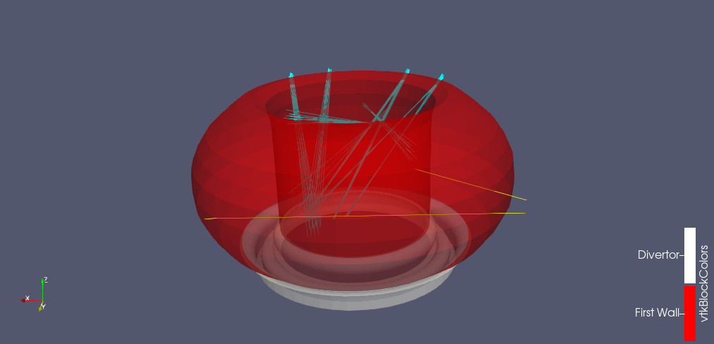
The interferometer lines of sight are added in yellow. Data provided by A. Medvedeva.
Loading the Magnetics Coil Positions
Navigate to Sources > IMAS Tools and select the Position Reader.
Enter the following URI in the
Enter URIfield of the Position reader plugin:imas:hdf5?path=/work/imas/shared/imasdb/ITER_MACHINE_DESCRIPTION/3/150100/5Since this URI only contains a single supported IDS for this reader, the magnetics IDS, it is automatically selected for you. You should see the magnetic coil names appear in the attribute array selection, select them all, and press
Apply.To visualize the positions, select the
Point Gaussianrepresentation under the Display properties section, and increase the Gaussian Radius to 0.05.Change the color of the coil positions to a color of choosing, by pressing
Editunder the coloring options. Here we use green.
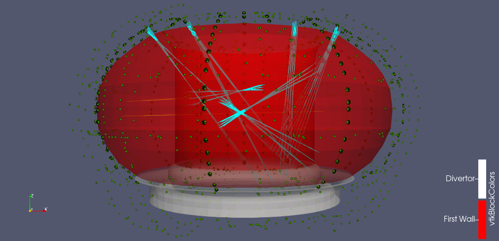
The magnetic coil positions are added in green. Data provided by M. Hosokawa.
Create an Animation with Orbiting Camera
Open the Time Manager under View > Time Manager
At the bottom besides the Animations tab, select Camera and Follow Path. Then press the plus icon to create a new camera animation.
Double-click the
Camera - RenderView1camera animation that you created. Select the first time value and selectCreate Orbit. Here, ensure the normal vector is set to 0,0,1.Increase the number of frames to 100 in the Time Manager.
Save the animation by going to File > Save Animation, enter a directory and name for the video, and in the Save Animation Options increase the frame rate to 20.
The resulting animation is shown below:
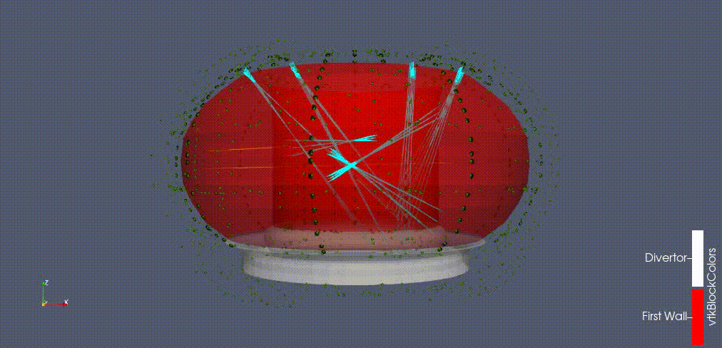
Animation of the multiple different types of ITER machine description data. Data provided by J. Artola.