JOREK Case¶

In this example, we will visualize a JOREK disruption case. A number of JOREK disruption cases are available on this confluence page (behind login wall). We will visualize the electron temperature from the plasma_profiles IDS and the corresponding current magnitude in the inner vacuum vessel of the wall IDS. We will create an animation to visualize how these change over time.

You can download the ParaView state file for this example here. However, we recommend that you manually follow the steps outlined below.

Loading the Electron Temperature¶

In this subsection, we load the JOREK grid and visualize the electron temperature on this grid.

The JOREK grid uses a combined finite-element and Fourier-series discretization. Bicubic finite elements describe fields in the poloidal plane, while a Fourier series handles variation in the toroidal direction. The standard GGD reader cannot process this grid structure, therefore, the JOREK reader was made available to load JOREK datasets. To load it, navigate to Sources > IMAS Tools and select the JOREK Reader.
Instead of loading the data set by entering the URI, we will now manually input the required fields. To do so, select the Enter pulse, run, .. option in the Data entry URI dropdown. Fill in the following fields, and then press Apply to load the URI:

Backend

HDF5

Database

ITER_DISRUPTIONS

Pulse

112111

Run

2

User

public

Version

4
Select the plasma_profiles/1 IDS in the IDS/Occurrence dropdown menu. Please refer to the confluence page for the meaning of different occurrences for this dataset.
Select Apply to load the plasma profiles GGD grid. Note: this dataset is quite large (~9GB) so it might take some time to load.
After the GGD grid is loaded, bring the grid into view by aligning the viewpoint in the positive Y direction using the following button: .
Select the Electrons Temperature from the attribute array selection window.
Select Apply to load the electron temperature values on the grid.
Select Electrons Temperature [eV] in the coloring dropdown to visualize the electron temperature.
Enable log scale coloring by selecting Edit under the Coloring section. In the Color Map Editor on the right, enable Use Log Scale When Mapping Data To Colors.
Set the N plane to 3 and the Phi range from 0 to 180 degrees in the Bezier interpolation settings.

Backend	HDF5
Database	ITER_DISRUPTIONS
Pulse	112111
Run	2
User	public
Version	4

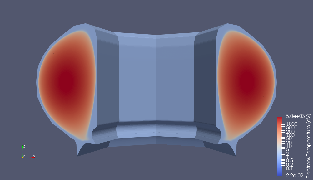
_images/jorek_electron_temp.png — JOREK GGD showing the electron temperature. Data provided by J. Artola.¶

Loading the Wall Current¶

In this subsection, we load the wall currents in the inner vacuum vessel using the GGD Reader and apply a clip mask.

Navigate to Sources > IMAS Tools and select the GGD Reader.
We will now load the same data entry as in the previous subsection, but we will enter it using the URI string option. To do so, enter the following URI in the Enter URI field of the GGD reader plugin, and press Apply:
```
imas:hdf5?user=public;pulse=112111;run=2;database=ITER_DISRUPTIONS;version=4
```
Select the wall IDS in the IDS/Occurrence dropdown menu.
Select Apply to load the wall grid.
Select J_total from the attribute array selection window.
Select Apply to load the current on the wall GGD grid.
Select Description_ggd J_total [A.m^-2] in the coloring dropdown and select Magnitude to visualize the total wall current.
As the wall shows an enclosed surface that is hard to see, apply a clip filter to the wall grid. To do this, select the clip filter: .
Set the normal vector to 0, -1, 0 and select Apply to apply the filter.
To distinguish between the wall currents and the electron temperature grid, change the wall current color map. Edit the color map, select Select a color map from default presets, and choose a different color map.

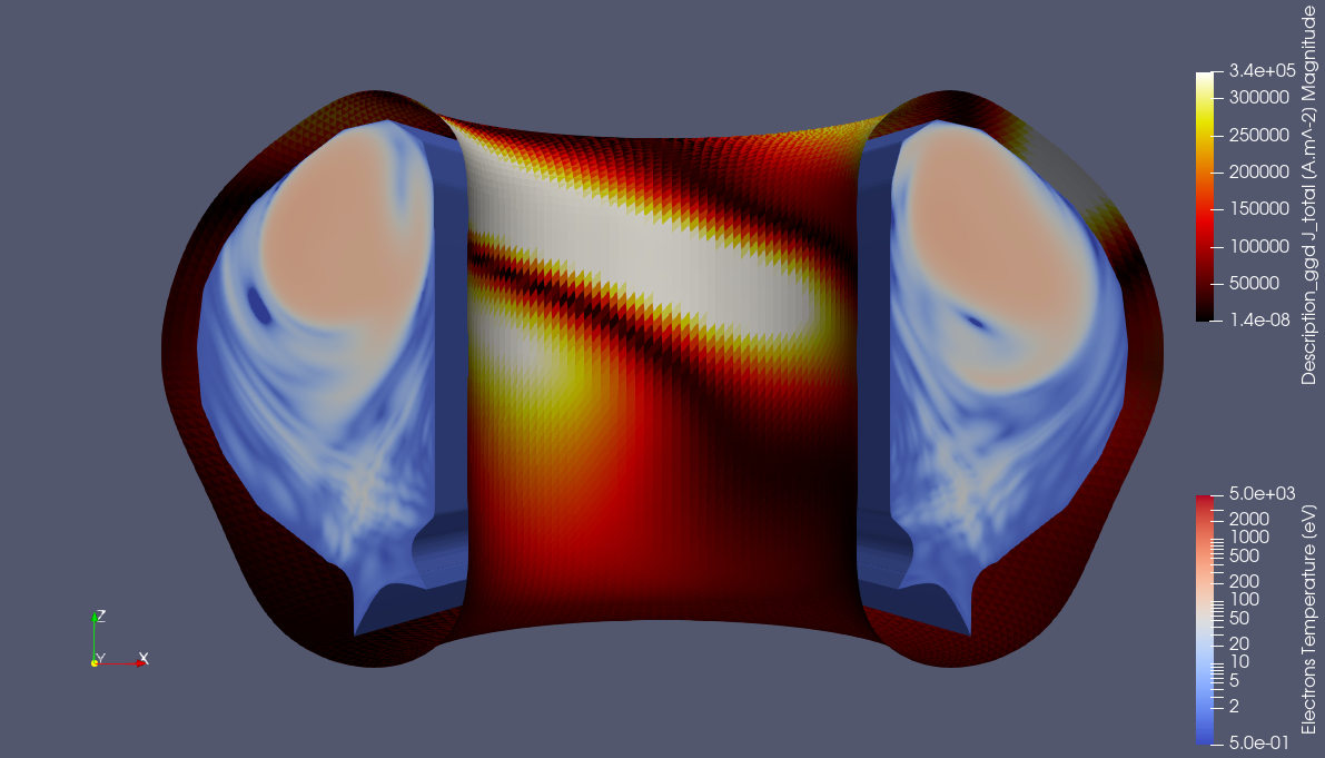
_images/jorek_wall_currents.png — JOREK GGD showing the electron temperature surrounded by total current in the inner vacuum vessel (`t=0.309984`). Data provided by J. Artola.¶

Temporal Interpolation and Animation¶

In this subsection, we create an animation of the loaded electron temperature and wall currents. We interpolate the time basis of both plugins to a linearly spaced basis.

To visualize the current time in the video, add a time value in the corner of the viewer using Sources > Annotation > Annotate Time. Press Apply to apply the time annotation source.
Select the JOREKReader and apply a Temporal Interpolator filter found under Filters > Temporal > Temporal Interpolator.
Set the Discrete Time Step Interval to 0.01, and select Apply to apply the temporal interpolation.
Now we will do the same for the wall currents. Select the created Clip filter and apply another Temporal Interpolator filter found under Filters > Temporal > Temporal Interpolator.
Set the Discrete Time Step Interval to 0.01, and select Apply to apply the temporal interpolation for the wall currents.
Right click on the clip filter in the pipeline, and deselect the Ignore Time checkbox.
Verify that both temporal interpolators are working by opening View > Time Manager and checking if the two temporal interpolators have the same number of time steps and that the time steps are of equal size.
Create an animation of the JOREK electron temperature and wall currents over time. Place the objects in the viewpoints in the desired orientation for the video. To create a video, go to File > Save Animation, provide a directory and a name for the video, and select OK.
In the pop-up window, video settings such as image resolution and compression can be changed. In this example, we set the frame rate to 5 and the frame window from 25 to 50. Press OK to start generating the animation. This may take a while.

The resulting animation is shown below:

_images/jorek.gif — Animation of the electron temperature and wall currents. Data provided by J. Artola.¶

Last update: 2026-03-11