JINTRAC case
In this example, we will visualize the electron temperature GGD of the edge profiles IDS, as well as the 1D core profiles. We will use the psi grid from the equilibrium IDS to map the 1D electron temperature profiles onto a 2D grid. By doing this, we can visualize the electron temperature both in the edge plasma and in the core in a single image.
You can download the ParaView state file for this example here. However, we recommend that you manually follow the steps outlined below.
Loading the Edge Profiles Electron Temperature
This subsection covers loading and visualizing the electron temperature in the edge plasma region from the edge_profiles IDS data.
Navigate to Sources > IMAS Tools and select the GGD Reader.
Enter the following URI in the
Enter URIfield of the GGD reader plugin, and pressApply:imas:hdf5?path=/work/imas/shared/TEST/simulations/test/8743dad6d7f211ef8fd59440c9e7706c/imasdb/iter/3/53298/2Select the edge_profiles IDS in the IDS/Occurrence dropdown menu.
Select
Applyto load the edge profiles GGD grid.After the GGD grid is loaded, bring the grid into view by aligning the viewpoint in the positive Y direction using the following button:
 .
.Select the
Electrons Temperaturefrom the attribute array selection window.Select
Applyto load the electron temperature values on the grid.Select
Electrons Temperature [eV]in the coloring dropdown to visualize the electron temperature.
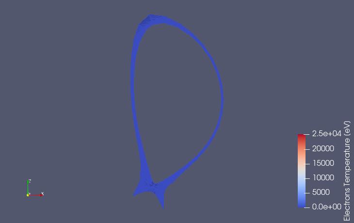
GGD grid of the edge profiles containing the electron temperature. Data provided by S.H. Kim.
Loading the Electron Temperature 1d Profile
This subsection covers loading the 1D electron temperature profile, and plotting it in a line chart with the normalized toroidal flux coordinate (rho_tor_norm) on the x-axis.
Navigate to Sources > IMAS Tools and select the 1D Profiles Reader.
Enter the following URI in the
Enter URIfield of the 1D Profiles reader plugin:imas:hdf5?path=/work/imas/shared/TEST/simulations/test/8743dad6d7f211ef8fd59440c9e7706c/imasdb/iter/3/53298/2Select the core_profiles IDS in the IDS/Occurrence dropdown menu.
Select
Applyto load the available core profiles.Select the
Electrons Temperaturefrom the attribute array selection window.Select
Applyto load the electron temperature 1D profile.To plot the 1D profile, we will apply a plotting filter. This can be found under Filters > Data Analysis > Plot Data. Select
Applyto apply the filter.In the filter properties, uncheck
Use Index For X Axisand in theX Array Namedropdown selectrho_tor_norm. Also uncheckrho_tor_normfrom the Series Parameters. You should now have a line chart of the electron temperature with the normalized toroidal flux coordinate on the x-axis.
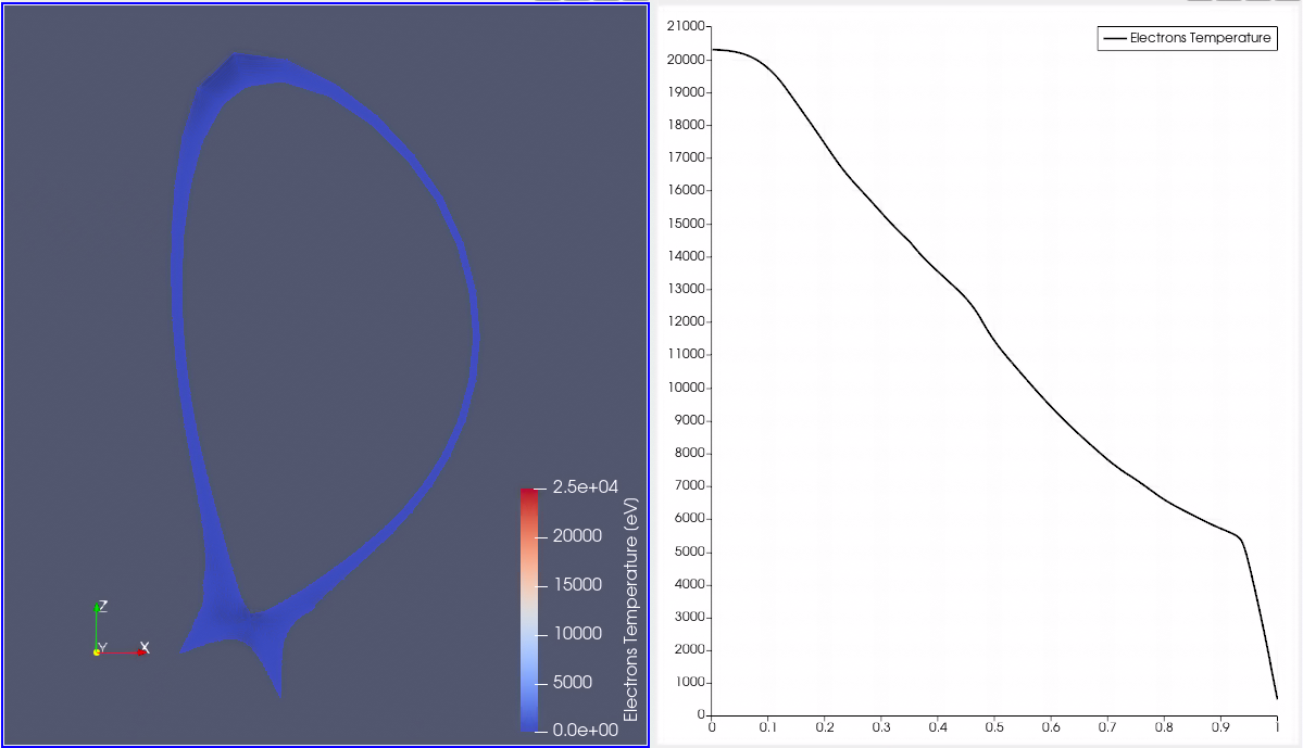
GGD grid of the edge profiles containing the electron temperature (left). 1D core profile of the electron temperature (right). Data provided by S.H. Kim.
Loading the Poloidal Flux 2D Profile
This subsection covers loading and visualizing the poloidal flux from the equilibrium IDS to create the 2D plane for mapping 1D profiles.
Navigate to Sources > IMAS Tools and select the 2D Profiles Reader.
Enter the following URI in the
Enter URIfield of the 2D Profiles reader plugin, and pressApply:imas:hdf5?path=/work/imas/shared/TEST/simulations/test/8743dad6d7f211ef8fd59440c9e7706c/imasdb/iter/3/53298/2Select the equilibrium IDS in the IDS/Occurrence dropdown menu.
Select
Applyto load the equilibrium 2D profiles.Select the
Psifrom the attribute array selection window.Select
Applyto load the poloidal flux values on the grid.Select
Psi [Wb]in the coloring dropdown to visualize the poloidal flux.Select the 1D Profiles Reader, and select the
Grid Psi
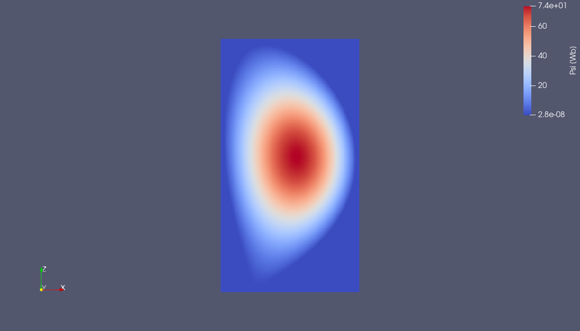
2D profile showing the poloidal flux. Data provided by S.H. Kim.
Mapping 1D Profiles onto 2D Equilibrium Grid
This subsection covers the mapping of the 1D electron temperature profile onto the 2D equilibrium grid to produce a 2D profile of the electron temperature.
Select the 1D Profiles Reader and apply the following filter: Filters > IMAS Tools > 1D Profiles Mapper.
In the pop-up window, we must select which source contains the psi grid and which contains the 1D profile. So select the 2D Profiles Reader for the psi grid, and the 1D Profiles Reader for the 1D profile. Press
OKto confirm the selection.Select
Applyto apply the 1D Profiles Mapper filter.Select the
Electrons Temperaturein theSelect 1D Profilesselection box. You will now see the 1D profile mapped onto a 2D grid.Values outside the valid psi range are colored yellow by default, but we can make them transparent instead. To do this, select
Editunder the Coloring section and set theNan Opacityto 0. You should now see that the 1D profile is mapped within the edge profiles of the GGD Reader.The data sets now have separate color bar ranges, so we can manually set these to the same range. For this, select the 1D Profiles Mapper filter and select the rescale to custom data range button:
 . Set the range from 0 to 25000.
Repeat the previous step for the GGD Reader, and remove the visibility of one of the colorbars, using the following button:
 .
.
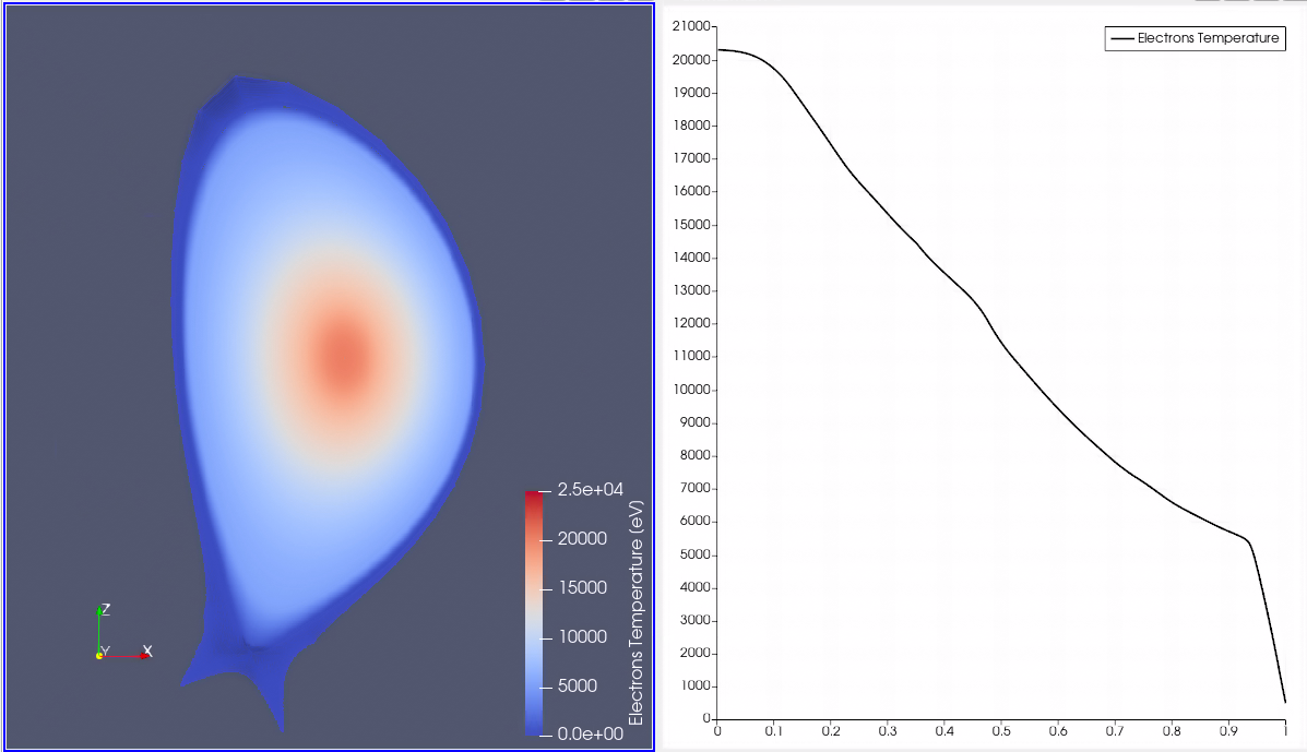
GGD grid of the edge profiles containing the electron temperature, the 1D core profile on the right as been mapped to 2D. Data provided by S.H. Kim.